
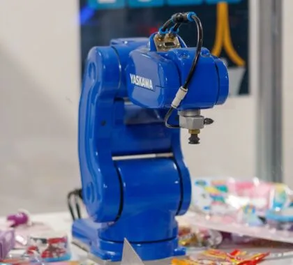
A line stops when a gripper misses a shifted part
A packaging cell in Ohio runs twelve hours a day. Every morning a new SKU arrives. The robot picks cartons from a conveyor. The cartons shift. The gripper misses. The line stops. A technician walks over. He jogs the robot. He adjusts the pick point. The line restarts. That walk costs forty minutes. It happens three times a shift.
The plant manager counts the cost. Three stops times forty minutes is two hours. Two hours times twelve shifts a week is twenty-four hours. Twenty-four hours times a loaded labor rate of two hundred dollars is four thousand eight hundred dollars a week. That is the arithmetic the owner checks every Friday.
Optical sensors feed fresh data to the control loop without stopping the robot
Cameras mounted on the robot wrist and above the conveyor stream pixel data to an edge computer. The edge computer runs a lightweight vision model. The model detects the carton corner in each frame. It computes the offset from the taught pick point. It sends a correction vector to the robot controller over the real-time fieldbus. The robot adjusts its trajectory mid-motion. The line does not stop. The technician does not walk.
This is the direct answer to the headline. Optical tech updates the robot’s AI on the fly by closing the perception-to-action loop at the edge. The robot keeps moving. The model keeps learning. The operator keeps watching output, not faults.
Why this matters for plants running mixed SKUs on shared cells
Contract packagers run fifty SKUs on one line. Each SKU has a different carton size, label position, and weight distribution. The old way: teach a recipe for each SKU. Store the recipe. Load the recipe at changeover. Hope the carton sits where the recipe expects it.
The new way: teach one baseline recipe. Let the optical system handle the variance. The vision model sees the carton. It measures the variance. It corrects the trajectory. The recipe stays static. The perception adapts.
This matters because changeover time drops. A changeover that took forty-five minutes now takes five. Five minutes to swap end-of-arm tooling. Zero minutes to retouch points. The plant gains forty minutes of production per changeover. Ten changeovers a week yields four hundred minutes. Four hundred minutes at two hundred dollars loaded rate is eight thousand dollars a week. The owner checks that number too.
What it looks like in practice — named steps and checkable arithmetic
Step one: mount a global-shutter camera on the robot wrist. Mount a second camera on a gantry above the conveyor. Both cameras trigger on the same encoder pulse. Cost: two industrial cameras at three thousand each. Two lenses at eight hundred each. Two cables and mounts at four hundred total. Hardware spend: eight thousand dollars.
Step two: install an edge computer in the cell cabinet. An industrial PC with a discrete GPU. Cost: four thousand dollars. Install the vision runtime. Connect cameras via GigE. Connect the PC to the robot controller via EtherCAT. Commissioning labor: sixteen hours at one hundred fifty dollars an hour. Labor spend: two thousand four hundred dollars.
Step three: collect baseline images. Run the line at reduced speed for two shifts. Save every frame with the encoder timestamp and the robot joint angles. Label the pick point in two hundred frames. Train a corner-detection model on that set. Training takes forty minutes on the edge GPU. Validation: run the model on a held-out set. Measure pixel error. Target: under two pixels at working distance.
Step four: deploy the model in inference mode. The runtime reads a frame, outputs a correction vector, sends it to the controller. The controller adds the vector to the taught path. The robot executes the corrected path. Latency budget: camera exposure plus transfer plus inference plus fieldbus write must stay under eight milliseconds. At eight milliseconds the robot moves six millimeters at two thousand millimeters per second. The correction lands before the gripper closes.
Step five: measure the result. Count stops before and after. Before: three stops per shift. After: zero stops per shift for carton shift. The four thousand eight hundred dollars a week in lost time returns to production. Payback on the fourteen thousand four hundred dollar install: three weeks.
The arithmetic uses numbers the plant already knows: stop frequency, stop duration, loaded labor rate, hardware quotes, labor rates. No survey. No benchmark. Just the owner’s spreadsheet.
How a business acts on it
Start with the cell that stops the most. Pull the stop log. Pick the top cause. If the cause is position variance that a camera can see, the optical loop fits. If the cause is a broken feeder or a jammed gripper, the optical loop does not fix it. Say plainly what automation cannot do: it cannot fix mechanical wear, it cannot invent a grasp strategy for a part it has never seen, it cannot override a safety stop.
Engage an integrator who has deployed edge vision on the same robot brand. Ask for a reference cell running the same cycle time. Ask for the latency log. Ask for the model retrain procedure when a new SKU arrives. The procedure should be: collect two hundred frames, label, retrain, validate, deploy. No robot code change.
Budget the install in the current quarter. Run the pilot on one cell. Measure stops per shift for four weeks. If the payback holds, scale to the next cell. The goal is not replacing staff. The goal is keeping the staff you have running production instead of chasing faults.
Alpha Edge builds the edge runtime and the model pipeline. We integrate with your robot controller and your fieldbus. We do not sell cameras. We do not sell robots. We sell the loop that keeps the robot moving when the part shifts. AI consulting for your operation starts with a stop log review and a latency budget. What we build includes the vision runtime, the training pipeline, and the fieldbus adapter for your controller.
Forward — the loop tightens as models shrink and fieldbuses speed up
Today the loop runs at one hundred twenty-five hertz on EtherCAT. Next year the same hardware runs at five hundred hertz on TSN. The model shrinks from fifty megabytes to five. The inference drops from four milliseconds to one. The correction lands earlier in the trajectory. The robot can adjust not just the pick point but the approach angle and the grip force.
The plant that installs the loop now owns the data stream. Every frame labeled. Every correction logged. That dataset becomes the training set for the next model. The next model handles not just carton shift but label skew, flap tuck, and tape variance. The line that stopped three times a shift stops zero times. The technician who walked the line now reviews the log and approves the new SKU recipe in five minutes.
The arithmetic compounds. Four thousand eight hundred dollars a week saved becomes eight thousand when the next variance class is covered. The install cost stays sunk. The marginal cost of the next model is labeling time and GPU hours. The owner checks the spreadsheet every Friday. The numbers keep moving in the right direction.